Solar wind
The Sun’s liberation velocity is written :
(1) 
We can compare this speed with the speed of sound calculated in the solar corona, which is composed mainly of hydrogen plasma at temperatures in the million Kelvin range:
(2) 
The Sun is mainly composed of hydrogen. We’ve just shown with simplistic arguments that, for a proton to escape the Sun’s gravitational pull, it must have a largely supersonic speed. And indeed, there is a continuous stream of plasma moving radially away from the Sun at supersonic speeds, known as the solar wind.
You can check it out, in real time, here: https://www.swpc.noaa.gov/products/real-time-solar-wind
The data displayed here are measured at the L1 Lagrange point by the DSCOVR satellite. The L1 Lagrange point is a “fixed” point, where an object can remain in equilibrium under the gravitational influences of the Sun and Earth. It is therefore, on an astronomical scale, much closer to the Earth than to the Sun.
The speed, displayed in violet in panel 4, and the temperature, displayed in green in panel 5, should enable the brave to verify that the solar wind is indeed supersonic.
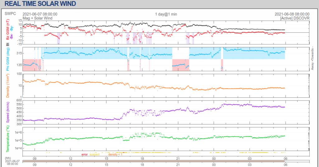
If we look at the top panel, we can see that one of the most important quantities in the solar wind is the magnetic field.
We can compare the order of magnitude of the magnetic energy per unit volume  , that of thermal energy
  and that of kinetic energy
  .
.
The solar wind is therefore a plasma transporting mainly kinetic energy, but also, in relatively equal proportions, thermal and magnetic energy. These calculations apply close to Earth.
Interaction with planets
Since the solar wind is supersonic, we expect its interaction with planets to lead to the formation of shocks. Not only is this the case, but it also leads to complex and distinct planetary environments from planet to planet. The Earth, for example, itself has a strong magnetic field, and its interaction with the solar wind leads to the formation of two boundaries: a (bow) shock and a magnetopause. Between the magnetopause and the bow shock lies the magnetogain, a dense, turbulent plasma zone, and behind the magnetopause lies the magnetosphere, where the magnetic field lines are attached to the Earth.
If we look again at the real-time data describing the solar wind plasma, we see that it is highly variable. This variability leads to frequent, and sometimes significant, changes in the structure of planetary environments. One of the quantities made clearly visible (in red) is the vertical component of the magnetic field:  . The reason this quantity is of particular interest is that, as early as 1961, it was identified as one of the determining factors in controlling solar wind/magnetosphere interaction. Indeed, when the interplanetary magnetic field has a negative component, this component directly opposes the Earth’s magnetic field, leading to favorable conditions for what is known as magnetic reconnection. The following diagram shows what happens:
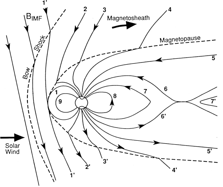
Field line 1′ (which is then only in the solar wind) connects to field line 1 (which is only connected to the Earth). They then become field lines 2 and 2′, with one foot in the solar wind and one on Earth. The ever-propagating solar wind drags these field lines (3, 3′, 4, 4′, 5 and 5′) and stretches them behind the Earth. There, they can be pushed against each other (6 and 6′) until they eventually go through a new magnetic reconnection episode (7 and 7′). During this reconnection episode, plasma particles can be accelerated and propagate along the field line 7, then 8. In this way, solar wind particles can enter the magnetosphere and deposit energy.
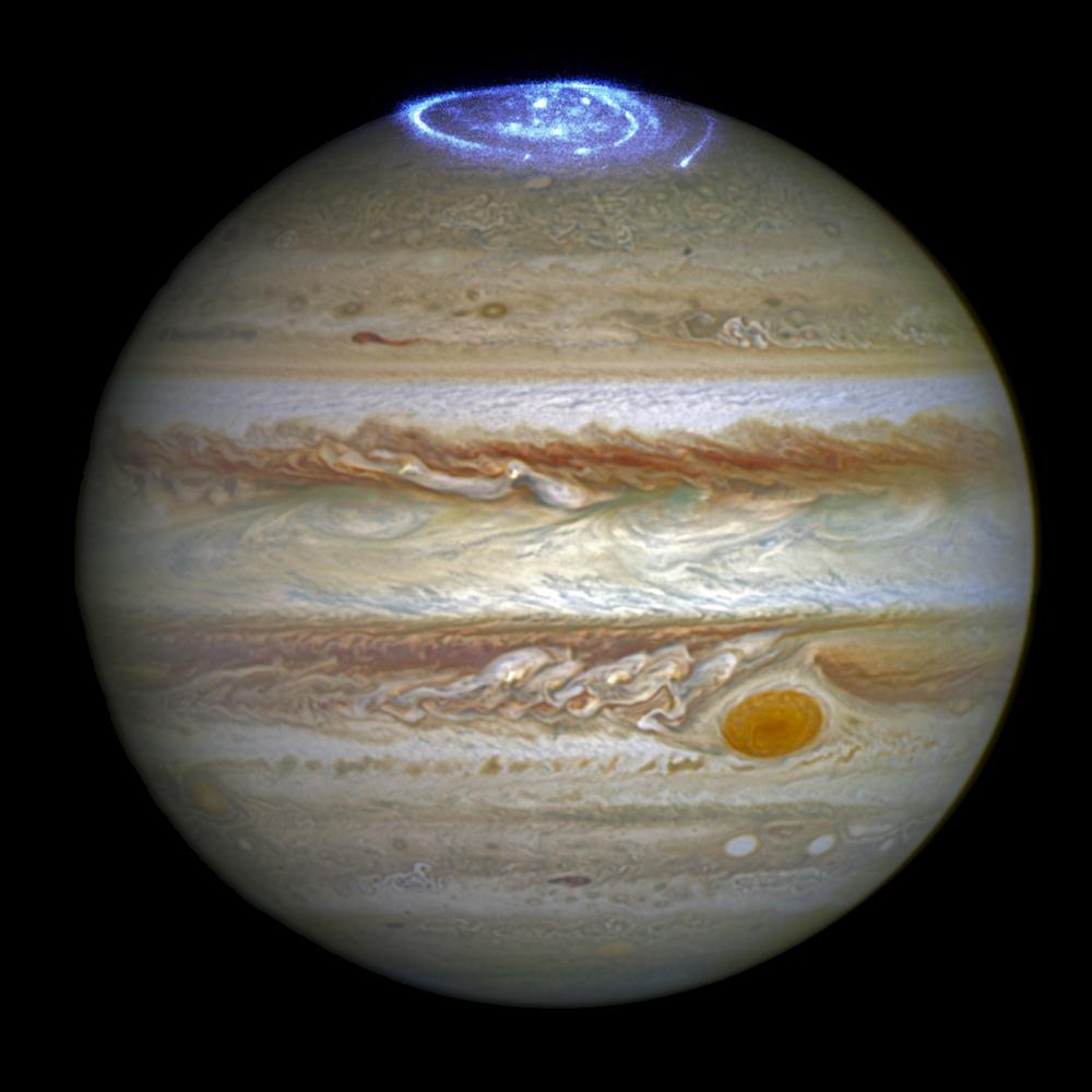
This complex process is, among other things, at the origin of the aurora borealis, which doesn’t just exist on Earth.
Magnetic reconnection
As mentioned above, when magnetic field lines of opposite polarity are pushed against each other, they can “reconnect”. Magnetic energy is thus efficiently converted into kinetic and thermal energy.
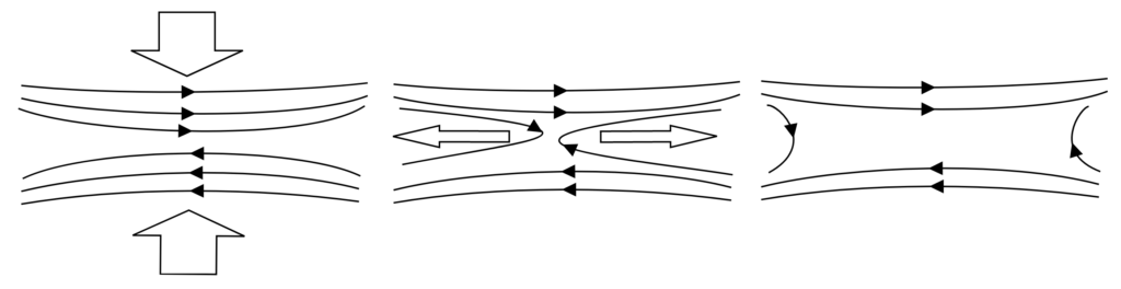
One of the first models of magnetic reconnection, called the Sweet-Parker model, calculates the reconnection rate, i.e. an estimate of the rate at which magnetic energy is converted into particle energy. The following brief presentation of the model uses notations common in plasma physics. Readers unfamiliar with the field should feel free to skip the equations and go straight to the conclusion.
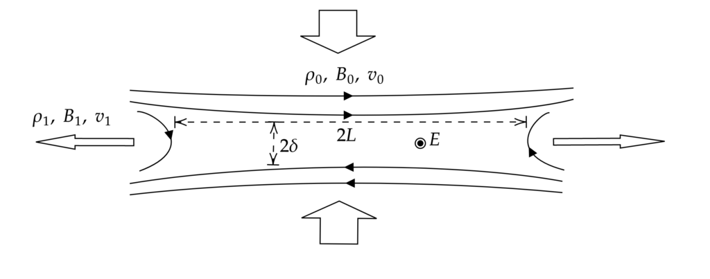
The assumptions made in this model are, on the one hand, those implicit in Figure 4: the model is 2D, the reconnection zone can be assimilated to a rectangle of length  and width
  , the electric field is constant inside, the reconnection is symmetrical…
(3) 
With a little algebra, we can calculate the reconnection rate, defined as the ratio of the incident plasma velocity to the Alfvén velocity in the incident plasma ( ):
):
(4) 
In the solar wind, we can estimate  , we can make the favorable assumption that the reconnection zone extends along the entire daytime part of the magnetopause, i.e.
  , where
  is the Earth’s radius. With
  and
and  , we estimate
  . We then find a very low reconnection rate:
(5) 
In reality, the observed reconnection rate is close to 0.1. The Sweet-Parker model, very useful for understanding the physics of magnetic reconnection, has very restrictive assumptions that don’t allow for good numerical predictions of reconnection rates.
Space plasma physics research
Many researchers are interested in the solar wind itself. For example, they may wonder whether and how energy changes from one type to another (for example, from magnetic to thermal, or from thermal to kinetic). We can look at the variable characteristics of the solar wind: is it slow? fast? particularly hot? The next question is the origin of these different types of solar wind: from which solar region do they originate? How are they formed? What types of waves do they contain?
We’re also interested in the interaction between the solar wind and the various planets:
Particularly with the Earth, since this interaction can have major consequences for certain human technologies (GPS, power lines, radio, etc.). For a long time, the big question was to find the interplanetary parameter(s) that controlled the strength of the solar wind/magnetosphere interaction. As we have seen, one answer is the value of . But this is too simple an answer to reflect the complex reality of this interaction. In particular, it can only explain (and even then only) the reconnection of field line 1′ with field line 2, in the previous figure. What about the reconnection between 6 and 6′? Other types of interaction? On the flanks of the magnetopause, for example? Nowadays, it’s more common to focus on classes of interplanetary structures: interplanetary coronal mass ejections, magnetic clouds, sheaths, shocks, Corotation Interaction Region, and their impact on the geomagnetic environment. There are at least two reasons for this. Firstly, it’s a more natural way of looking at the complexity of interactions. Secondly, it is hoped (and actively pursued) that we will be able to predict their appearance using optical images of the Sun, which will give us much more time to take preventive measures on Earth.
The interaction of the solar wind with other planets can be very different, as their properties are quite different from those of the Earth. Mercury, for example, which is not magnetized like the Earth, is the focus of a research program around the BepiColombo mission, which will orbit Mercury in 2025. Today, we have plasma data from satellites around the various planets and moons of the solar system, associated with many mysteries to be solved.
The question of magnetic reconnection is one of the major issues occupying researchers in space plasma physics. And it’s not the only one, since it’s a fundamental phenomenon in plasma physics, as much at work in fusion plasmas as in the search for the origin of cosmic rays. In the solar system, as we’ve seen, it appears at two points in the interaction between the solar wind and the Earth’s geomagnetic environment; but it is also one of the phenomena behind solar flares. All the assumptions made in the Sweet-Parker model above are debatable, and are the subject of research programs: 3D reconnection, asymmetric reconnection, non-magnetohydrodynamic effects, reconnection for a compressible plasma, etc.